The Data Mining involves a systematic analysis of data sets. It gives a meaning to the approachable data. Data mining is the study of collecting, cleaning, processing, analyzing, and gaining useful insights from data. Especially nowadays, Decision tree learning algorithm has been successfully used in expert systems in capturing knowledge. The aim of this article is to show a brief description about decision tree. This paper clarified the decision tree meaning, split criteria, popular decision tree algorithms, advantages and disadvantages of decision tree. At the end of the paper, training set is given and a sample of decision tree is created using Quinlan’s ID3.

Introduction

This article explains the meaning of decision tree, gives an information about the place of decision tree in data mining. Also, this paper involves an information about tree size, splitting criteria, entropy an information gain.

The classes of an instances set (or training set), we can use several algorithms to discover the way the attributes-vector of the instances behaves, to estimate the classes for new instances.  Decision trees, which originally derived from logic, management and statistics, are today highly effective tools in other areas such as text mining, information extraction, machine learning, and pattern recognition.

According to Rokach and Maimon, Decision trees offer many benefits:

• Versatility for a wide variety of data mining tasks, such as classification, regression, clustering and feature selection
• Self-explanatory and easy to follow (when compacted)
• Flexibility in handling a variety of input data: nominal, numeric and textual
• Adaptability in processing datasets that may have errors or missing values
• High predictive performance for a relatively small computational effort
• Available in many data mining packages over a variety of platforms
• Useful for large datasets (in an ensemble framework)

Decision tree has a learning algorithm like ID3, C4.5, CART, CHAID, QUEST, Cal5, Fact, LMDT, T1, Public: mars.  In this paper chose to explain only four of them: ID3, C4.5 , CHAID and QUEST.

ID3  algorithm has chosen as a project in this paper because of the simplicity.

Data Mining with the Decision Tree

According to Aggarwal, Decision trees are a classification methodology, wherein the classification process is modeled with the use of a set of hierarchical decisions on the feature variables, arranged in a tree-like structure. [1]

According to Bhargava, Sharma and Bhargava & Mathuria, A decision tree is a decision support system that uses a tree-like graph decisions and their possible after-effect, including chance event results, resource costs, and utility. A Decision Tree, or a classification tree, is used to learn a classification function which concludes the value of a dependent attribute (variable) given the values of the independent (input) attributes (variables). This verifies a problem known as supervised classification because the dependent attribute and the counting of classes (values) are given [2].

The decision tree consists of nodes that form a rooted tree, meaning it is a directed tree with a node called “root” that has no incoming edges. All other nodes have exactly one incoming edge. A node with outgoing edges is called an internal or test node. All other nodes are called leaves (also known as terminal or decision nodes) [3].

In a decision tree, each internal node splits the instance space into two or more sub-spaces according to a certain discrete function of the input attributes values. In the simplest and most frequent case, each test considers a single attribute, such that the instance space is partitioned according to the attribute’s value. In the case of numeric attributes, the condition refers to a range [3].

Each leaf is assigned to one class representing the most appropriate target value. Alternatively, the leaf may hold a probability vector indicating the probability of the target attribute having a certain value. Instances are classified by navigating them from the root of the tree down to a leaf, according to the outcome of the tests along the path. Figure 1 describes a decision tree that reasons whether or not a potential customer will respond to a direct mailing. Internal nodes are represented as circles, whereas leaves are denoted as triangles [3].

Note that this decision tree incorporates both nominal and numeric attributes. Given this classifier, the analyst can predict the response of a potential customer (by sorting it down the tree), and understand the behavioral characteristics of the entire potential customers population regarding direct mailing [3].

Each node is labeled with the attribute it tests, and its branches are labeled with its corresponding values [3].

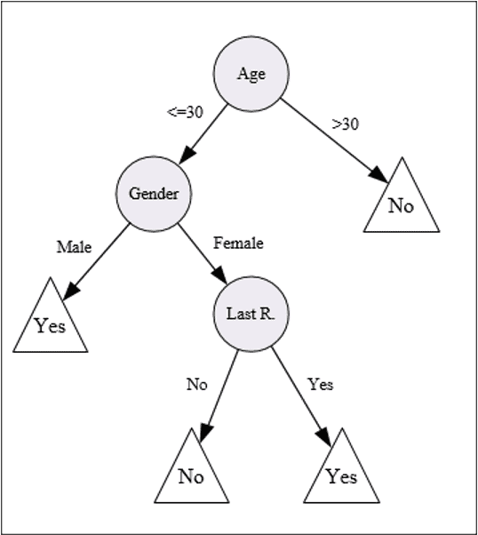
One of the paths in Figure 1 can be transformed into the rule: “If customer age is is less than or equal to or equal to 30, and the gender of the customer is “Male” – then the customer will respond to the mail”.

The resulting rule set can then be simplified to improve its comprehensibility to a human user, and possibly its accuracy [4].

2.1 Split Criteria

The goal of the split criterion is to maximize the separation of the different classes among the children nodes. In the following, only univariate criteria will be discussed. Assume that a quality criterion for evaluating a split is available. The design of the split criterion depends on the nature of the underlying attribute [1]:

• Binary attribute: Only one type of split is possible, and the tree is always binary. Each branch corresponds to one of the binary values.
• Categorical attribute: If a categorical attribute has r different values, there are multiple ways to split it. One possibility is to use an r-way split, in which each branch of the split corresponds to a particular attribute value. The other possibility is to use a binary split by testing each of the 2r − 1 combinations (or groupings) of categorical attributes, and selecting the best one. This is obviously not a feasible option when the value of r is large. A simple approach that is sometimes used is to convert categorical data to binary data with the use of the binarization approach. In this case, the approach for binary attributes may be used.
• Numeric attribute: If the numeric attribute contains a small number r of ordered values (e.g., integers in a small range [1, r]), it is possible to create an r-way split for each distinct value. However, for continuous numeric attributes, the split is typically performed by using a binary condition, such as x ≤ a, for attribute value x and constant a.

Many of the aforementioned methods requires the determination of the “best” split from a set of choices. Specifically, it is needed to choose from multiple attributes and from the various alternatives available for splitting each attribute. Therefore, quantifications of split quality are required. These quantifications are based on the same principles as the feature selection criteria [1]:

2.1. 1 Error rate:

Let p be the fraction of the instances in a set of data points S belonging to the dominant class. Then, the error rate is simply 1−p. For an r-way split of set S into sets S1 . . . Sr, the overall error rate of the split may be quantified as the weighted average of the error rates of the individual sets Si, where the weight of Si is |Si|. The split with the lowest error rate is selected from the alternatives [1].

2.1.2 Gini index:

The Gini index G(S) for a set S of data points may be computed on the class distribution p1 . . . pk of the training data points in S [1].

The overall Gini index for an r-way split of set S into sets S1 . . . Sr may be quantified as the weighted average of the Gini index values G(Si) of each Si, where the weight of Si is |Si| [1].

The split with the lowest Gini index is selected from the alternatives. The CART algorithm uses the Gini index as the split criterion. [1]

2.1. 3 Entropy

The entropy measure is used in one of the earliest classification algorithms, referred to as ID3 [1 ].

As in the case of the Gini index, the overall entropy for an r-way split of set S into sets S1 . . . Sr may be computed as the weighted average of the Gini index values G(Si) of each Si, where the weight of Si is |Si|.

Lower values of the entropy are more desirable. The entropy measure is used by the ID3 and C4.5 algorithms. [1].

The information gain is closely related to entropy, and is equal to the reduction in the entropy E(S) − Entropy-Split(S ⇒ S1 . . . Sr) as a result of the split. Large values of the reduction are desirable. At a conceptual level, there is no difference between using either of the two for a split although a normalization for the degree of the split is possible in the case of information gain. Note that the entropy and information gain measures should be used only to compare two splits of the same degree because both measures are naturally biased in favor of splits with larger degree. For example, if a categorical attribute has many values, attributes with many values will be preferred. It has been shown by the C4.5 algorithm that dividing the overall information gain with the normalization factor of helps in adjusting for the varying number of categorical values [1].

The aforementioned criteria are used to select the choice of the split attribute and the precise criterion on the attribute. For example, in the case of a numeric database, different split points are tested for each numeric attribute, and the best split is selected [1].

2.2 Tree Size

Naturally, decision makers prefer a decision tree that is not complex since it is apt to be more comprehensible. Furthermore tree complexity has a crucial effect on its accuracy [5]. Usually the tree complexity is measured by one of the following metrics: the total number of nodes, total number of leaves, tree depth and number of attributes used. Tree complexity is explicitly controlled by the stopping criteria and the pruning method that are employed [6].

2.3 Popular Decision Trees Induction Algorithms

All of these algorithms are using splitting criterion and pruning methods. In this part, algorthms of ID3, C4.5 and CHAID are explained [8].

2.3.1 ID 3

The ID3 algorithm is considered to be a very simple decision tree algorithm [7]. Using information gain as a splitting criterion, the ID3 algorithm ceases to grow when all instances belong to a single value of a target feature or when best information gain is not greater than zero. ID3 does not apply any pruning procedure nor does it handle numeric attributes or missing values. The main advantage of ID3 is its simplicity. Due to this reason, ID3 algorithm is frequently used for teaching purposes [8].

Disadvantages of ID3

Disadvantages are given below [8]:

• ID3 does not guarantee an optimal solution, it can get stuck in local optimums because it uses a greedy strategy. To avoid local optimum, backtracking can be used during the search.
• ID3 can overfit to the training data. To avoid overfitting, smaller decision trees should be preferred over larger ones. This algorithm usually produces small trees, but it does not always produce the smallest possible tree.
• ID3 is designed for nominal attributes. Therefore, continuous data can be used only after converting them to nominal bins.

2.3.2 C4 5

C4.5, an evolution of ID3, presented by the same author uses gain ratio as splitting criteria. [9]. The splitting ceases when the number of instances to be split is below a certain threshold. Error-based pruning is performed after the growing phase. C4.5 can handle numeric attributes [8].

C4.5 algorithm provides several improvements to ID3. The most important improvements are [8]:

• 5 uses a pruning procedure which removes branches that do not contribute to the accuracy and replace them with leaf nodes.
• 5 allows attribute values to be missing (marked as ?).
• 5 handles continuous attributes by splitting the attribute’s value range into two subsets (binary split). Specifically, it searches for the best threshold that maximizes the gain ratio criterion. All values above the threshold constitute the first subset and all other values constitute the second subset.

Nevertheless, a recent comparative study that compares C4.5 with J48 and C5.0 [10] indicates that C4.5 performs consistently better (in terms of accuracy) than C5.0 and J48 in particular on small datasets [8].

2.3.3 CHAID

Starting from the early Seventies, researchers in applied statistics developed procedures for generating decision trees [11]. Chi-squared- Automatic-Interaction-Detection (CHIAD) was originally designed to handle nominal attributes only. For each input attribute ai, CHAID finds the pair of values in Vi that is least significantly different with respect to the target attribute. The significant difference is measured by the p value obtained from a statistical test. The statistical test used depends on the type of target attribute. An F test is used if the target attribute is continuous; a Pearson chi-squared test if it is nominal; and a likelihood ratio test if it is ordinal [8].

For each selected pair of values, CHAID checks if the p value obtained is greater than a certain merge threshold. If the answer is positive, it merges the values and searches for an additional potential pair to be merged. The process is repeated until no significant pairs are found. The best input attribute to be used for splitting the current node is then selected, such that each child node is made of a group of homogeneous values of the selected attribute. Note that no split is performed if the adjusted p value of the best input attribute is not less than a certain split threshold [8].

Chi-squared Automatic Interaction Detection. At each step, CHAID chooses the independent (predictor) variable that has the strongest interaction with the dependent variable. Categories of each predictor are merged if they are not significantly different with respect to the dependent variable [12].

2.3.4 QUEST

The Quick, Unbiased, Efficient Statistical Tree (QUEST) algorithm supports univariate and linear combination splits [13]. For each split, the association between each input attribute and the target attribute is computed using the ANOVA F-test or Levene’s test (for ordinal and continuous attributes) or Pearson’s chi-square (for nominal attributes). An ANOVA F-statistic is computed for each attribute. If the largest F-statistic exceeds a predefined threshold value, the attribute with the largest F-value is selected to split the node. Otherwise, Levene’s test for unequal variances is computed for every attribute. If the largest Levene’s statistic value is greater than a predefined threshold value, the attribute with the largest Levene value is used to split the node. If no attribute exceeded either threshold, the node is split using the attribute with the largest ANOVA F-value. Quick, Unbiased, Efficient Statistical Tree. A method that is fast and avoids other methods’ bias in favor of predictors with many categories. QUEST can be specified only if the dependent variable is nominal [12].

	CHAID*	QUEST
Chi-square-based**	X
Surrogate independent (predictor) variables		X
Tree pruning		X
Multiway node splitting	X
Binary node splitting		X
Influence variables	X
Prior probabilities		X
Misclassification costs	X	X
Fast calculation	X	X

*Includes Exhaustive CHAID.

**QUEST also uses a chi-square measure for nominal independent variables [12].

2. 4 Advantages and Disadvantages of Decision Trees

Several advantages of the decision tree as a classification tool have been pointed out in the literature [8]:

1. Decision trees are self–explanatory and when compacted they are also easy to follow. In other words if the decision tree has a reasonable number of leaves, it can be grasped by non–professional users. Furthermore decision trees can be converted to a set of rules. Thus, this representation is considered as comprehensible.
2. Decision trees can handle both nominal and numeric input attributes.
3. Decision tree representation is rich enough to represent any discrete-value classifier.
4. Decision trees are capable of handling datasets that may have errors.
5. Decision trees are capable of handling datasets that may have missing values.
6. Decision trees are considered to be a nonparametric method. This means that decision trees have no assumptions about the space distribution and the classifier structure.
7. When classification cost is high, decision trees may be attractive in that they ask only for the values of the features along a single path from the root to a leaf.

On the other hand, decision trees have such disadvantages as [8]:

1. Most of the algorithms (like ID3 and C4.5) require that the target attribute will have only discrete values.
2. As decision trees use the “divide and conquer” method, they tend to perform well if a few highly relevant attributes exist, but less so if many complex interactions are present. One of the reasons for this is that other classifiers can compactly describe a classifier that would be very challenging to represent using a decision tree. A simple illustration of this phenomenon is the replication problem of decision trees [14]. Since most decision trees divide the instance space into mutually exclusive regions to represent a concept, in some cases the tree should contain several duplications of the same sub-tree in order to represent the classifier. For instance if the concept follows the following binary function: y = (A1 \ A2) [ (A3 \ A4) then the minimal univariate decision tree that represents this function is illustrated in Figure 2 Note that the tree contains two copies of the same subt-ree.
3. The greedy characteristic of decision trees leads to another disadvantage that should be pointed out. This is its over–sensitivity to the training set, to irrelevant attributes and to noise make decision trees especially unstable: a minor change in one split close to the root will change the whole subtree below [9].

4. The fragmentation problem causes partitioning of the data into smaller fragments. This usually happens if many features are tested along the path. If the data splits approximately equally on every split, then a univariate decision tree cannot test more than O(logn) features. This puts decision trees at a disadvantage for tasks with many relevant features. Note that replication always implies fragmentation, but fragmentation may happen without any replication.
5. Another problem refers to the effort needed to deal with missing values [15]. While the ability to handle missing values is considered to be advantage, the extreme effort which is required to achieve it is considered a drawback. The correct branch to take is unknown if a feature tested is missing, and the algorithm must employ special mechanisms to handle missing values. In order to reduce the occurrences of tests on missing values, C4.5 penalizes the information gain by the proportion of unknown instances and then splits these instances into subtrees. CART uses a much more complex scheme of surrogate features.
6. The myopic nature of most of the decision tree induction algorithms is reflected by the fact that the inducers look only one level ahead. Specifically, the splitting criterion ranks possible attributes based on their immediate descendants. Such strategy prefers tests that score high in isolation and may overlook combinations of attributes. Using deeper lookahead strategies is considered to be computationally expensive and has not proven useful.

3-Application

Training Set: Products with accessories

The data set follows an example of attribute selection measure, information gain (ID3/C4.5). We will examine the products sold in the first quarter at the company

63 systems are sold in total.

No	Type	Plant	Turnover	Domestic	Kiosk
1	A	<=5	Low	yes	no
2	A	<=5	Low	yes	no
3	B	5…10	Medium	yes	yes
4	A	<=5	Medium	yes	no
5	A	<=5	High	yes	no
6	B	>10	Medium	yes	yes
7	A	<=5	Medium	yes	yes
8	A	<=5	Medium	yes	no
9	C	<=5	Medium	yes	yes
10	B	<=5	High	no	no
11	B	<=5	High	no	no
12	B	<=5	High	yes	yes
13	A	<=5	Low	yes	no
14	A	<=5	Low	yes	yes
15	B	5…10	High	no	no
16	A	<=5	High	no	yes
17	C	<=5	High	no	no
18	C	<=5	High	no	no
19	C	5…10	High	no	no
20	B	<=5	High	no	no
21	A	<=5	High	no	no
22	A	<=5	High	no	no
23	C	<=5	High	yes	yes
24	B	<=5	Low	yes	yes
25	C	<=5	Medium	yes	yes
26	C	<=5	Medium	yes	yes
27	A	5…10	Medium	yes	no
28	B	5…10	High	no	no
29	B	5…10	High	no	no
30	C	<=5	Low	yes	yes
31	B	5…10	High	no	no
32	C	<=5	Medium	yes	yes
33	B	<=5	Medium	no	no
34	B	<=5	Medium	no	no
35	A	<=5	Medium	no	no
36	A	5…10	Medium	yes	no
37	B	>10	Medium	yes	yes
38	C	<=5	Medium	yes	yes
39	C	<=5	Medium	yes	yes
40	A	<=5	Medium	yes	no

 

No	Type	Plant	Turnover	Domestic	Kiosk
41	C	<=5	Low	yes	yes
42	A	<=5	Medium	yes	no
43	C	<=5	Medium	yes	yes
44	B	<=5	Medium	yes	yes
45	A	<=5	Medium	yes	no
46	B	<=5	Low	yes	yes
47	A	<=5	High	yes	no
48	B	5…10	Low	no	no
49	B	5…10	Medium	yes	yes
50	A	<=5	High	no	no
51	A	<=5	High	yes	yes
52	A	<=5	High	no	yes
53	B	5…10	High	no	no
54	A	<=5	Low	yes	no
55	A	<=5	High	no	no
56	A	<=5	High	yes	no
57	C	>10	High	no	no
58	B	<=5	Medium	no	no
59	B	>10	High	yes	yes
60	A	<=5	Medium	yes	yes
61	A	<=5	Low	yes	yes
62	C	>10	High	no	no
63	A	<=5	High	no	no

 

P= Buys Product with accessories = “yes”

N= Buys Product with accessories = “no”

 

Type	pi	ni	I(pi,ni)
A	7	20	0,8256265
B	9	12	0,9852281
C	10	5	0,9182958
Plant	pi	ni	I(pi,ni)
<=5	21	26	0,9918208
5…10	2	9	0,6840384
>10	3	2	0,9709506
Turnover	pi	ni	I(pi,ni)
Low	6	5	0,9940302
Medium	14	11	0,9895875
High	6	21	0,7642045
Domestic	pi	ni	I(pi,ni)
yes	24	14	0,949452
no	2	23	0,4021792

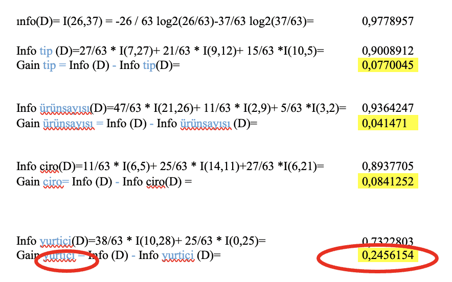
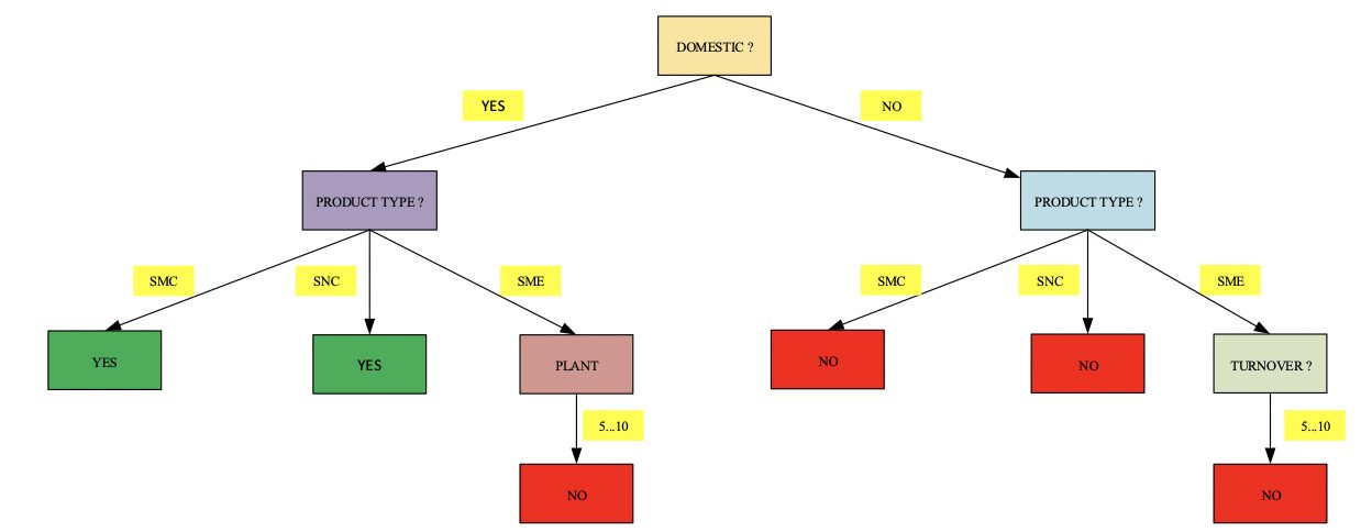
Biggest gain is chosen.  It means that first split is “domestic.” (Domestic yes and domestic no)

• For Domestic – yes;

No	Domestic	Type	Plant	Turnover	Kiosk
1	yes	A	<=5	Low	no
2	yes	A	<=5	Low	no
3	yes	B	5…10	Medium	yes
4	yes	A	<=5	Medium	no
5	yes	A	<=5	High	no
6	yes	B	>10	Medium	yes
7	yes	A	<=5	Medium	yes
8	yes	A	<=5	Medium	no
9	yes	C	<=5	Medium	yes
10	yes	B	<=5	High	yes
11	yes	A	<=5	Low	no
12	yes	A	<=5	Low	yes
13	yes	C	<=5	High	yes
14	yes	B	<=5	Low	yes
15	yes	C	<=5	Medium	yes
16	yes	C	<=5	Medium	yes
17	yes	A	5…10	Medium	no
18	yes	C	<=5	Low	yes
19	yes	C	<=5	Medium	yes
20	yes	A	5…10	Medium	no
21	yes	B	>10	Medium	yes
22	yes	C	<=5	Medium	yes
23	yes	C	<=5	Medium	yes
24	yes	A	<=5	Medium	no
25	yes	C	<=5	Low	yes
26	yes	A	<=5	Medium	no
27	yes	C	<=5	Medium	yes
28	yes	B	<=5	Medium	yes
29	yes	A	<=5	Medium	no
30	yes	B	<=5	Low	yes
31	yes	A	<=5	High	no
32	yes	B	5…10	Medium	yes
33	yes	A	<=5	High	yes
34	yes	A	<=5	Low	no
35	yes	A	<=5	High	no
36	yes	B	>10	High	yes
37	yes	A	<=5	Medium	yes
38	yes	A	<=5	Low	yes

 

P= Buys Product with accessories=”yes”

N= Buys Product with accessories=“no”

 

Tip	pi	ni	I(pi,ni)
A	5	14	0,8314744
B	9	0	0
C	10	0	0
Plant	pi	ni	I(pi,ni)
<=5	19	12	0,9629004
5…10	2	2	1
>10	3	0	0
Turnover	pi	ni	I(pi,ni)
Low	6	4	0,9709506
Medium	14	7	0,9182958
High	4	3	0,9852281

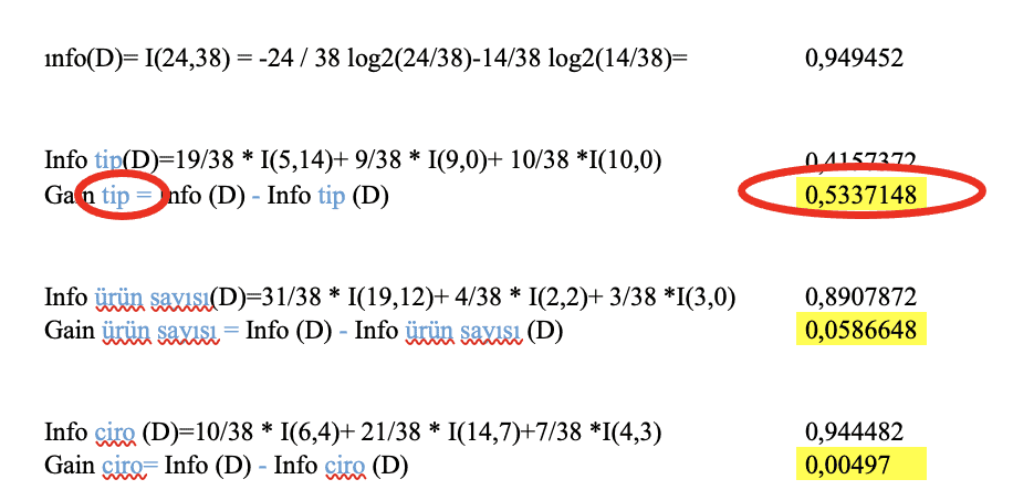
Biggest gain is chosen.  It means that second split is “type” (A,B,C) after “domestic – yes”

• For Type (A,B,C)

Domestic	Type	Plant	Turnover	Kiosk
yes	A	<=5	Low	no
yes	A	<=5	Low	no
yes	A	<=5	Medium	no
yes	A	<=5	High	no
yes	A	<=5	Medium	yes
yes	A	<=5	Medium	no
yes	A	<=5	Low	no
yes	A	<=5	Low	yes
yes	A	5…10	Medium	no
yes	A	5…10	Medium	no
yes	A	<=5	Medium	no
yes	A	<=5	Medium	no
yes	A	<=5	Medium	no
yes	A	<=5	High	no
yes	A	<=5	High	yes
yes	A	<=5	Low	no
yes	A	<=5	High	no
yes	A	<=5	Medium	yes
yes	A	<=5	Low	yes

 

P= Buys Product with accessories=“ “yes”

N= Buys Product with accessories=“ “no”

 

Ürün Sayısı	pi	ni	I(pi,ni)
<=5	5	12	0,873981
5…10	0	2	0
>10	0	0	0

 

Ciro	pi	ni	I(pi,ni)
Düşük	2	4	0,9182958
Orta	2	7	0,7642045
Yüksek	1	3	0,8112781

Domestic	Type	Plant	Turnover	Kiosk
yes	C	<=5	Medium	yes
yes	C	<=5	High	yes
yes	C	<=5	Medium	yes
yes	C	<=5	Medium	yes
yes	C	<=5	Low	yes
yes	C	<=5	Medium	yes
yes	C	<=5	Medium	yes
yes	C	<=5	Medium	yes
yes	C	<=5	Low	yes
yes	C	<=5	Medium	yes

 

For C Type

P= Buys Product with accessories=“ “yes”

N= Buys Product with accessories=“ “no”

 

Domestic	Type	Plant	Turnover	Kiosk
yes	B	5…10	Medium	yes
yes	B	>10	Medium	yes
yes	B	<=5	High	yes
yes	B	<=5	Low	yes
yes	B	>10	Medium	yes
yes	B	<=5	Medium	yes
yes	B	<=5	Low	yes
yes	B	5…10	Medium	yes
yes	B	>10	High	yes

 

For B Type

P= Buys Product with accessories=“ “yes”

N= Buys Product with accessories=“ “no”

• For Plant

Domestic	Type	Plant	Turnover	Kiosk
yes	A	5…10	Medium	no
yes	A	5…10	Medium	no

P= Buys Product with accessories=“ “yes”

N= Buys Product with accessories=“ “no”

 

Domestic	Type	Plant	Turnover	Kiosk
yes	A	<=5	Low	no
yes	A	<=5	Low	no
yes	A	<=5	Medium	no
yes	A	<=5	High	no
yes	A	<=5	Medium	yes
yes	A	<=5	Medium	no
yes	A	<=5	Low	no
yes	A	<=5	Low	yes
yes	A	<=5	Medium	no
yes	A	<=5	Medium	no
yes	A	<=5	Medium	no
yes	A	<=5	High	no
yes	A	<=5	High	yes
yes	A	<=5	Low	no
yes	A	<=5	High	no
yes	A	<=5	Medium	yes
yes	A	<=5	Low	yes

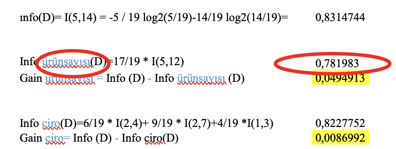
This split is not regular, so pruning is applied.

• For Domestic-No

Domestic	Type	Plant	Turnover	Kiosk
no	B	<=5	High	no
no	B	<=5	High	no
no	B	5…10	High	no
no	A	<=5	High	yes
no	C	<=5	High	no
no	C	<=5	High	no
no	C	5…10	High	no
no	B	<=5	High	no
no	A	<=5	High	no
no	A	<=5	High	no
no	B	5…10	High	no
no	B	5…10	High	no
no	B	5…10	High	no
no	B	<=5	Medium	no
no	B	<=5	Medium	no
no	A	<=5	Medium	no
no	B	5…10	Low	no
no	A	<=5	High	no
no	A	<=5	High	yes
no	B	5…10	High	no
no	A	<=5	High	no
no	C	>10	High	no
no	B	<=5	Medium	no
no	C	>10	High	no
no	A	<=5	High	no

 

P= Buys Product with accessories=“ “yes”

N= Buys Product with accessories=“ “no”

 

Type	pi	ni	I(pi,ni)
A	2	6	0,8112781
B	0	5	0
C	0	12	0
Plant	pi	ni	I(pi,ni)
<=5	2	14	0,5435644
5…10	0	7	0
>10	0	2	0
Turnover	pi	ni	I(pi,ni)
Low	0	1	0
Medium	0	4	0
High	2	18	0,4689956

 

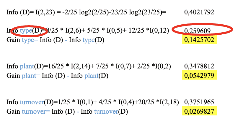
The biggest gain is chosen. “type” (A, B, C)

• For Type ;

Domestic	Type	Plant	Turnover	Kiosk
no	A	<=5	High	yes
no	A	<=5	High	no
no	A	<=5	High	no
no	A	<=5	Medium	no
no	A	<=5	High	no
no	A	<=5	High	yes
no	A	<=5	High	no
no	A	<=5	High	no

 

P= Buys Product with accessories=“ “yes”

N Buys Product with accessories=“ “no”

 

Plant	pi	ni	I(pi,ni)
<=5	2	6	0,8112781
5…10	0	0	0
>10	0	0	0

 

Turnover	pi	ni	I(pi,ni)
Low	0	0	0
Medium	0	1	0
High	2	5	0,8631206

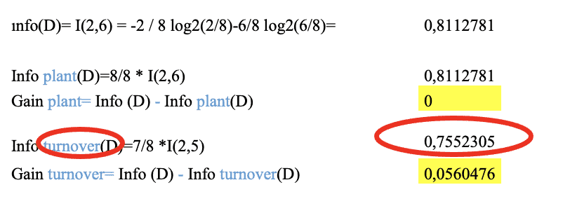
Domestic	Type	Plant	Turnover	Kiosk
no	C	<=5	High	no
no	C	<=5	High	no
no	C	5…10	High	no
no	C	>10	High	no
no	C	>10	High	no

 

For C Type
P= Buys Product with accessories=“ “yes”	0
N= Buys Product with accessories=“ “no”	5

 

Domestic	Type	Plant	Turnover	Kiosk
no	B	<=5	High	no
no	B	<=5	High	no
no	B	5…10	High	no
no	B	<=5	High	no
no	B	5…10	High	no
no	B	5…10	High	no
no	B	5…10	High	no
no	B	<=5	Medium	no
no	B	<=5	Medium	no
no	B	5…10	Low	no
no	B	5…10	High	no
no	B	<=5	Medium	no

• For B Type

P= Buys Product with accessories=“ “yes”	0
N= Buys Product with accessories=“ “no”	12

• For Turnover

Domestic	Type	Turnover	Plant	Kiosk
no	A	Medium	<=5	no

 

Domestic	Type	Turnover	Plant	Kiosk
no	A	High	<=5	yes
no	A	High	<=5	no
no	A	High	<=5	no
no	A	High	<=5	no
no	A	High	<=5	yes
no	A	High	<=5	no
no	A	High	<=5	no

This split is not regular, so pruning is applied.

After abovementioned calculation, decision tree consists of the following.

4-Conclusion

This paper presents the definition of decision trees, advantages and disadvantages.

Also, this paper gives an approaches of decision tree with the ID3, C4.5, CHAID, and QUEST; their advantages and disadvantages. The main advantage of ID3 is its simplicity. Due to this reason, ID3 algorithm is frequently used for teaching purposes. C4.5 algorithm is an evolution of ID3 and this uses gain ratio as splitting criteria. Chi-squared-Automatic-Interaction-Detection (CHIAD) was originally designed to handle nominal attributes only. CHAID handles missing values by treating them all as a single valid category. CHAID does not perform pruning. The Quick, Unbiased, Efficient Statistical Tree (QUEST) algorithm supports univariate and linear combination splits. QUEST has negligible bias and yields a binary decision tree. Ten-fold cross-validation is used to prune the trees.

Zeynep Ayça Gürel, Electrical Engineer – Quality Assurance

5-REFERENCES

[1] Aggarwal, C. C. (2015). Data mining: the textbook

[2] Bhargava, N., Sharma, G., Bhargava, R., & Mathuria, M. (2013). Decision tree analysis on j48 algorithm for data mining. Proceedings of International Journal of Advanced Research in Computer Science and Software Engineering, 3(6).

[3] Rokach, L., & Maimon, O. (2005). Decision trees. In Data mining and knowledge discovery handbook (pp. 165-192). Springer, Boston, MA.

[4] Quinlan, J.R., Simplifying decision trees, International Journal of Man-Machine Studies, 27, 221-234, 1987.

[5] Breiman, L., Friedman, J., Olshen, R., & Stone, C. (1984). Classification and regression trees. Wadsworth Int. Group, 37(15), 237-251.

[6] Rokach, L., & Maimon, O. Z. (2008). Data mining with decision trees: theory and applications (Vol. 69). World scientific.

[7] Quinlan J. R., Induction of decision trees, Machine Learning 1:81–106, 1986.

[8] Rokach, L., & Maimon, O. (2015). Data mining with decision trees–Theory and Applications 2nd Edition. Series in Machine Perception and Artificial Intelligence, 81, 328.

[9] Quinlan, J. R., C4.5: Programs for Machine Learning, Morgan Kaufmann, Los Altos, 1993.

[10] Moore S. A., Daddario D. M., Kurinskas J. and Weiss G. M., Are decision trees always greener on the open (source) side of the fence?, Proceedings of DMIN, pp. 185–188, 2009.

[11] Kass G. V., An exploratory technique for investigating large quantities of categorical data, Applied Statistics 29(2):119–127, 1980.

[12] IBM SPSS Decision Trees 19 by SPSS Inc. 1989, 2010.

[13] Loh W. Y., and Shih X., Split selection methods for classification trees, Statistica Sinica 7:815–840, 1997.

[14] Pagallo, G. and Huassler, D., Boolean feature discovery in empirical learning, Machine Learning, 5(1): 71-99, 1990.

[15] Friedman, J., Kohavi, R., Yun, Y. 1996. Lazy decision trees. Proceedings of the Thirteenth National Conference on Artificial Intelligence. (pp. 717-724).