Introduction

Understanding fundamental concepts such as Active Power, Reactive Power, Apparent Power, and Power Factor is crucial for any electrical engineer who wants to establish a solid foundation in power systems. This Excel-based study will be helpful in understanding these basic power concepts.

This work, in addition to strengthening your theoretical knowledge, also provides tips on using Microsoft Excel as a powerful tool for visualizing and analyzing electrical power systems.

Data Entry in Excel: Enter data into the following cells in our Excel model to analyze power dynamics:

• Cell B2: Enter Voltage Amplitude. (The system is set to operate at a constant frequency of 50 Hz)
• Cell D2: Enter Current Amplitude.
• Cell C3: Specify the Power Factor, which can be between 0 and 1.

Observing Results and Visualizations:

After entering the data, the Excel model offers real-time visualizations and calculations that facilitate an understanding of how electric power components interact:

• Cell D3 (Phase Delay Angle): View the delay angle between current and voltage, which shows the effect of the Power Factor on the system.
• Power Triangle Visualization: Observe changes in the amplitudes of Active, Reactive, and Apparent Power. This helps visualize the interrelation among these components in a power system.
• Calculated Power Values: Clear values for Reactive, Apparent, and Active Power are presented alongside the power triangle.
• Sinusoidal Waveforms: Visualize the sinusoidal waveforms of voltage and current with the delay angle depending on the power factor.
• Analysis of Active Power Components: Discover the positive and negative components of Active Power that arise depending on the angle between current and voltage.
• Effective Active Power Total: Discover that Effective Active Power emerges as the sum of its positive and negative components.

Practical Examples Analyzing System Behavior with Different Power Factors

Example 1: Purely Resistive System

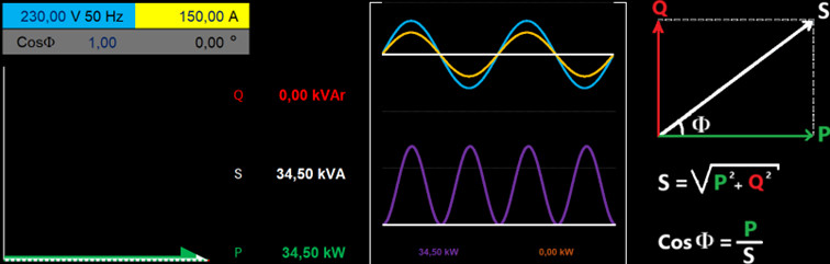
Input data:

• Voltage: 230 Volts
• Current: 150 Amperes
• CosPhi: 1.0

Observations:

• Phase Delay Angle: 0 degrees — no delay (angular difference) between voltage and current.
• System Characteristic: Purely Resistive
  • Active Power: 34.5 kW
  • Apparent Power: 34.5 kVA
  • Reactive Power: 0 kVAr
• The voltage-current sinusoidal waveform also shows no delay between current and voltage.
• All active power is generated in the positive alternation area; no active power is generated in the negative alternation area.
• The Total Active Power value is calculated as 34.5 kW.

What Is Unbalanced Current? Calculating in Excel

Example 2: Resistive + Reactive System

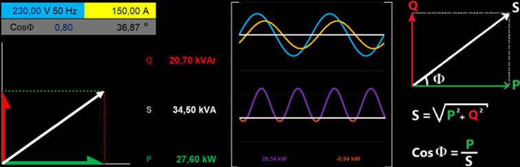
Input data:

• Voltage: 230 Volts
• Current: 150 Amperes
• CosPhi: 0.8

Observations:

• Phase Delay Angle: 36.87 degrees — there is a delay (angular difference) between voltage and current.
• System Characteristic: Resistive + Reactive
  • Active Power: 27.6 kW
  • Apparent Power: 34.5 kVA
  • Reactive Power: 20.7 kVAr
• The voltage-current sinusoidal waveform shows the current lagging behind the voltage.
• A large amount of active power is generated in the positive alternation area, with a small amount in the negative alternation area.
• The Total Active Power value is calculated as 28.54 – 0.94 = 27.6 kW.

Example 3: Purely Reactive System

Purely Reactive SystemInput data:

• Voltage: 230 Volts
• Current: 150 Amperes
• CosPhi: 0.0

Observations:

• Phase Delay Angle: 90.00 degrees — there is a delay (angular difference) between voltage and current.
• System Characteristic: Purely Reactive.
  • Active Power: 0 kW
  • Apparent Power: 34.5 kVA
  • Reactive Power: 34.5 kVAr
• The voltage-current sinusoidal waveform shows the current 90 degrees behind the voltage.
• Active power is generated in both the positive and negative alternation areas.
• The Total Active Power value is calculated as 10.98 – 10.98 = 0.0 kW.

Conclusion

To facilitate the understanding of basic power concepts through visualization, you can download and use the attached Excel file on your computer to experiment and experience these concepts.

Excel Document

You can download the Excel file by clicking here.